


How to Freeze/Pin Columns and Rows in Google Sheets
Organization is the key to accomplishing any given tasks on time. A working area kept in order makes a voluminous work seems easy to manage; this includes the data you’re working on your computer, specifically in Google Sheets. While it may be difficult to keep track of everything once numerous rows and columns are filled, organization is still possible when you learn the process of freezing or pinning certain rows and columns in the sheet.
Freezing or pinning the rows and columns in Google Sheets can make updating each of them very easy and at the most time-saving manner. When you learn the tips on how to do it correctly, you will see how scrolling over the entire document you’re working on can be so stress-free.
Ready to start your work? Here are the three simple steps on how to freeze or pin rows and columns in Google Spreadsheet:
- Choose the Google Sheet you want to edit and open it.
- Select the column(s) you want to freeze.
- Click the View menu, then choose Freeze. Select the number of columns you want to freeze (i.e. 1 column, 2 columns, or a range of columns).
If you wish to unfreeze the columns, you may simply repeat the steps above and select No Columns instead of Freeze.

How to Hyperlink a Cell in Google Sheets
A quick way to access an external webpage from your Google Sheet is through a hyperlink. It’s been a common practice of many who want their own web-pages linked to other sites.
When you create hyperlinks in your sheets, all you need to do is click on them and you will be led to a specific web page.
Basically, here are the steps in creating a hyperlink in Google Sheets based from the Google Support Site:
- Find and open your spreadsheet.
- Click the cell in the spreadsheet where you wish the link to appear.
- Choose from the following options:
- Click the “Insert” drop-down menu and select Link.
- Click the link icon in the toolbar.
- Right click in the spreadsheet and select the Insert link option.
- Use the Ctrl + K keyboard shortcut (Cmd + K on a Mac).
- In the “Text” field that appears, type or edit the text you’d like displayed in the cell containing the link. Leave the field blank if you want the full URL to be displayed in your spreadsheet.
- In the “Link” field, you can either paste a URL or email address, or type in the field to begin a search of relevant links across web content and your Google Drive files. You may also click Find more below the search results to browse additional options.
- Click Apply.

How to Download Google Sheets
Your Google sheets may be downloaded through very simple steps. Here’s how:
- Open Google Docs.
In your web browser, go to https://docs.google.com/ which will access the Google Docs page integrated when you’re logged into your Google Account. Otherwise, just type your email address and enter your password when asked to.
- Select a document you wish to download.
- Click File. You can find this option in the upper-life side portion of the page.
- Select Download as from thedrop-down menu wherein you will be prompted by a pop-menu.
- Choose a specific format for the file.
You can either click Microsoft Word (.docx) which converts the file into a Word document or PDF document (.pdf) if you want it to be in PDF format. Right after, you will get a prompt to download your Google Docs file to download onto your computer. Take note, however, you may need confirmation to download or select which location your file will be saved when you download it to your computer.
How to Add Columns and Rows in Google Sheets
Another helpful function you can use when working on Google Sheets is to add rows or columns to your current spreadsheet to keep it more organized. You can add rows or columns as many as you prefer them and it’s very easy to learn.
You can start by going to the Google Sheets home page from your browser. Choose which specific spreadsheet you want to insert rows or columns by opening it.

Then, click on a particular cell where you wish to have a column or row inserted to. Right after, from the toolbar, select the “Insert” option.

You will then have several options to choose from for inserting rows and columns into your spreadsheet. You can choose to insert them from different positions, either from the top or below for rows, and either to the left or right of the selected cell for columns.

You also have the discretion to add just one row or column at a time, or highlight as many cells you would want to insert. For instance, you can choose to highlight two vertical cells to insert two rows or highlight two horizontal cells to insert columns.

You can likewise add rows and columns from the from the right-click context menu by highlighting the cell you want to insert them next to, right-click your selected cells then select either “Insert Rows” or “Insert Columns.”

When using the right-click option, rows and columns automatically will be inserted to the left side of the selected cells.
And that’s it! It is just so easy to add or insert rows/columns to your sheet.
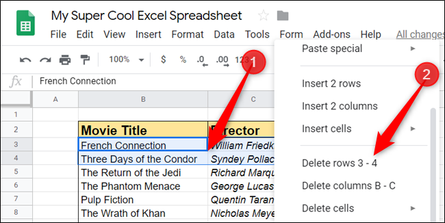
How to Remove Rows or Columns
Once again, same as the initial step for adding or inserting rows or columns, go to Google Sheets in your browser and open the spreadsheet you want to have a column and/or row deleted or removed.
Highlight the specific cell in the row or column that you wish to be deleted. Just right-click on it and you may choose either “Delete Row” or “Delete Column.”

To save time and effort, if there is a need to delete a number of rows or columns, just right-click on it and choose your preferred cells to be removed and delete them.
Whether you want to add or remove rows and columns from the spreadsheet you are working on, you will definitely learn the process fast and you can complete any tasks you have on Google Sheets in a very short span of time.
How to Alphabetize and Order a Google Sheet
One primary function we often use in Google Sheet is arranging the terms or data in an alphabetical order. It’s more interesting to know that the same process may be used when we need to have the data sorted by their numerical value or to arrange the dates.
It’s all made possible by the SORT function in Google Sheets.
To illustrate, for instance, and you need to have the data (name of countries) in a set of a column alphabetized quickly.
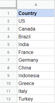
Here is a formula you can follow:
=SORT(A2:A12)

You need to put in mind, however, that the SORT function may be limited in a lot of ways. In situations wherein you need to sort a single column data alphabetically then you just need to put in that formula as illustrated above.
How to Add Borders to Cells in Google Sheets
The convenience that Google Sheets offer to its users is just unlimited. It indeed serves its purpose when it comes to organizing tasks. Just like how it offers the option to add borders to cells in your sheets.
Adding borders to cells in your sheets can be a great help for you to view and read all the data you’ve filled in multiple cells easily. Here’s the list you can follow to add cell borders:
- Select the cell or cells you want to make the neccesary changes in format.

2. From the drop-down menu, choose the Borders button then select the desired border option.

3. You will then see the new cell borders.

How to Make Alternating Colors in a Google Sheet
Lastly, you can have your sheet colored for you to easily spot any reference you need when preparing for a certain report from your spreadsheet. It can be found in the fill color option.
First, you need to select the cell or cells you want to make changes with. Then, from the toolbar, you must locate and select the fill color button.

Right after, choose your desired color from the drop-down, as illustrated below:

You will then see the new fill color.

Some truly rattling work on behalf of the owner of this site, perfectly great written content. Daniele Michal Gemina
Thank you very much.
If you want more help like this please join our email list.